Movements in monkeys & mice

September 15, 2022

Today’s paper, current on the preprint server, is, “Neural cognitive signals during spontaneous movements in the macaque.” It is co first-authored by Sébastien Tremblay and Camille Testard at the McGill University. The main take home message of the paper is that in primate prefrontal cortex, neurons are modulated by both task variables and uninstructed movements, and that this mixed selectivity does not hinder the ability to decode variables of interest.

Pupil, face and body movement data were critical for the interpretation.

Approach: the authors measured neural activity from 4,414 neurons in Area 8 using Utah Arrays (chronically implanted electrodes). Animals were engaged in a visual association task in which they had to keep a cue in mind over a delay period while they waited for a target to instruct them about what to do. The authors took videos of the animals and labeled these using DeepLabCut so that they could examine the collective influence on neural activity of task variables, instructed movements (that they trained the animal to make) and uninstructed movements. They also measured pupil diameter. The data visualizations for both of these are quite nice! I mean look at the pupil!

In mice and monkeys, uninstructed movements account for a lot of single trial variance.

In addition to a number of nice analyses about the mixed selectivity of neurons for parameters like the location and identity of the target, the authors deployed an encoding model to compare the relative influence on neural activity of a number of parameters. Fortuitously, they took advantage of existing code in my lab developed by Simon Musall and Matt Kaufman for our 2019 paper. The reason this was so helpful is that it allows the reader to easily compare findings from 2 different experiments. This is really unusual in a paper!! We need more of this in the field! In this case it totally facilitated a cross-species comparison which is not usually very easy to do. They found, as we did, that uninstructed movements have a big impact on neural acetivity (left). These movements included the cheeks, nose, arms, pupil, and the raw motion energy from the video. For me, it was super cool to see the contribution of movements to single trial activity in such a different area and species. Importantly, they tested their ability to decode parameters of interest given the magnitude of movement-driven activity. They could! This is reminiscent of previous observations from Carsen Stringer, who argued that in mouse V1, movement driven activity is mostly orthogonal to stimulus-driven activity, preventing movements from contaminating V1’s representation of the stimulus. 

Skeptic’s corner: This paper was really a pleasure to read and my main confusion came from the framing of the result in the discussion. The authors found that task variables accounted for a bit more single-trial variance in their experiment than ours. I agree with their assessment, which is that it is hard to know how to interpret this difference because the recordings in this paper are from an area with strong visually-driven activity by exactly the sorts of images they used. We instead measured activity cortex-wide. Given this methodological difference, I was a bit puzzled by the statement that, “Mice and primates diverged ~100 million years ago, such that findings from mice research sometimes do not translate to nonhuman primates.” I mean, that statement is for sure true, but this particular paper seemed instead like evidence for the opposite- it points to shared computations in diverse brains. Along the same lines, they say “Perhaps in nonhuman primates, association cortical areas evolved neural machinery independent from movement circuits, such that cognitive signals can be fully dissociated from the immediate sensorymotor environment.” I was again a bit confused because the take home of the paper seemed to be that movements modulated neural activity. The issue at hand here might be the extent to which the movement signals “sully” the waters: disrupt the ability of a downstream area to decode a task parameter of interest. Here, decoding is preserved even in the face of movement, which is cool. But again, I think the situation appears to be the same in mice and monkeys- the movements live in an orthogonal subspace so don’t get in the way of decoding. Maybe Carsen Stringer will weigh in here- I feel like this is exactly what her paper showed in mice, albeit using a different analysis.

A final nugget: Figure S9 shows a 95% prediction of the correct target based on facial movements alone and even before the animal knows where the target will appear on the screen. Wow!

Thanks to Matt Kaufman and Simon Musall for a fun discussion on this topic.

Neural activity patterns for PT and IT pyramidal subtypes during a sensorimotor task

By Felicia Davatolhagh & Anne Churchland

Today’s paper is Cortical Glutamatergic Projection Neuron Types Contribute to Distinct Functional Subnetworks by Hemanth Mohan, Xu An, Hideki Kondo, Shengli Zhao, Katherine S. Matho, Simon Musall, Partha Mitra, and Z. Josh Huang. In this paper, the authors reveal that pyramidal tract (PT) and intratelencephalic (IT) pyramidal neuron subtypes have distinct neural responses across cortex during different behavioral states and as an animal processes sensory information. 

Approach: The authors recorded large-scale calcium responses of PT and IT neurons across the dorsal cortex using widefield imaging and genetic targeting. Novel mouse driver lines Fezf2 and Plxnd1 were crossed onto an Ai148 reporter line to selectively express GCaMP6f in PT and IT neurons. This combination permitted the authors to monitor neural activity of distinct cell types through the intact cleared skull to understand the differences between PT and IT neural activity. 

Take-home messages: The main message taken from the paper is the observation that PT and IT neurons have distinct activation patterns during various aspects of behavior. The authors find differences during wakeful resting, spontaneous movements, and sensory stimulation (i.e. visual, whisker, and orofacial). Furthermore, they reveal that PT and IT neurons are dynamically tuned to different sensorimotor components of a hand-assisted pellet feeding task. Specifically, these pyramidal subtypes form functional subnetworks with activation patterns spanning distinct regions. PT neurons were activated across parietal and frontal cortex, while IT neurons were activated in orofacial primary sensory cortex (frontolateral posterior node; FLP) and in primary and secondary motor cortex (frontolateral anterior node; FLA). These subnetworks were further dissected using a laser scanning method to bilaterally inhibit regions of the dorsal cortex, finding that parietofrontal and frontolateral subnetworks serve distinct roles in the feeding behavior paradigm.

Skeptics corner: The authors found preferential activation of IT neurons over PT neurons in response to sensory inputs including visual, orofacial and whisking. This was surprising to us since given our observations of sensory-locked responses in both PT and IT neurons (Musall et al. 2022). It is important to note that a direct comparison of these figures is difficult since ΔF/F is used in Mohan et al, while the figure in Musall et al shows the output of an encoding model. Another potential contributor to this difference in findings may be the use of dissimilar sensory modalities (somatosensory vs. auditory) or behavioral state (passive vs. engaged in a task). Nonetheless, this raises interesting questions about the circumstances under which PT neurons are modulated by sensory signals.

Mixed selectivity seen in OFC clusters that are defined by temporal response patterns

I recently read this preprint from Christine Constantinople’s lab. The paper is about encoding of decision variables in frontal cortex and I read it (and wrote this post) alongside Abby Muthusamy, a UCLA PhD student in my lab (left).

Approach: The authors used a value-based decision making task in which rats were simultaneously presented with randomized auditory clicks and visual flashes indicating reward probability and volume available at each side port. Upon training, rats reliably selected the side port with the greater subjective reward value; they’re good at it! The team performed k-means clustering and conditional clustering on single-unit recordings from the lOFC to interpret neural encoding of task variables (stimulus, reward attributes, reward outcome, reward history, and choice).

Take home message: Both clustering methods revealed 5 subpopulations of neurons (clusters) in the lOFC with distinct temporal profiles. Importantly, these subpopulations were not functionally distinct: all 5 clusters were modulated by all task variables. This was clear both from a rigorous analysis and also from a GLM, the results of which are quite clear and also beautifully presented (see Figure). Back to the main message: remember here that “mixed selectivity” refers to a property of single neurons. It means that they are modulated by more than one variable. Here, we are looking at clusters rather than single neurons, so must use the term loosely. Still, the overall finding appears very much in favor of mixed selectivity, in keeping with observations of mixed selectivity in non-human primates for economic decision variables in frontal cortex. The results of the current preprint potentially conflict with another paper in rats observing categorical encoding and NOT mixed selectivity, making me wonder what’s really going on in the frontal cortex!

A final interesting point: one cluster was transiently “enriched” for signals relating to reward history, and these popped up just before the animal’s choice. This suggests that subpopulations in the lOFC not only mix value and stimulus signals, but also previous and current outcomes before choice, just when the rat needs them most.

Skeptic’s corner: The authors utilized two clustering methods, which strengthened their argument for 5 subpopulations arising in the lOFC during this task. Still, we would have liked to see a method that explicitly tested if clusters exist at all (such as PAIRS from Raposo et al. 2014, or the even better MCMC employed in this paper; it allows ones to identify both pure-selective and non-selective components). The downside with methods like k-means is that they find clusters whether they are there are not, rather than asking whether clusters are present vs. absent.

Also, we found it curious that  Cluster 3 (Fig. 1E, 2D) contained two seemingly distinct subpopulations of neurons, one peaking at trial start and the other peaking immediately prior to choice. We wonder whether the early peaking neurons within Cluster 3 should belong to Cluster 1 instead?

How can sensory stimuli have a shrinking effect on decision-making?

It’s been a while since we’ve updated the ORACLE! We are still reading papers on the preprint server, but our ability to write about them got a bit slowed down: COVID happened, and then we moved to UCLA! We’ll try to ramp back up now that we are getting settled. The paper below is one that I read with James Roach, a postdoc in my lab, and our conversations about it shaped my thinking.

The paper: Attractor dynamics gate cortical information flow during decision-making; Arseny Finkelstein, Lorenzo Fontalan, Michael Economo, Nuo Li, Sandro Romani & Karel Svoboda.

This crew aimed to uncover how sensory information can have a differential impact on actions depending on when in the course of a decision it is presented. They developed this approach to tackle this problem: they presented trained mice with distractors (photostimulation to primary somatosensory cortex) at different times during a delay period that preceded a response period. Behaviorally, stimuli presented earlier had the biggest impact, indicating that later stimuli were “gated out” or, were somehow prevented from impacting the neural activity that drove the licking response. To determine the mechanism of this gating, the authors measured neural activity in a region of the frontal cortex, the anterior lateral motor cortex (ALM). These measurements demonstrated that neural activity likewise became more robust to distractors over time. To me, this was the main take-home: the sensory stimuli still impacted ALM activity, but the choice-related dynamics became progressively more robust over the trial so that these same stimulus-driven deflections had a smaller effect.

In an artificial network trained up to generate outputs matching the mean responses of neurons he recorded in ALM. In the artificial network, attractor dynamics stabilized the activity of the units, making them more robust to perturbations. A key feature of this network was a “ramping input”, based on some observations in the data.

I liked 3 things about this paper. First, the behavioral paradigm is good: the diminishing effect of distractors over time is very robust. Also, this diminishing behavioral effect stands in contrast to the non-attenuation of the distractors in either S1 or ALM. Second, the data analysis was compelling. Specifically, the authors used a targeted dimensionality reduction approach to interpret the activity of area ALM in light of both sensory and movement planning signals. This analysis made it possible to compare ALM and S1 despite differing sensory responses in those two areas. Finally, the inclusion of an artificial network was an important addition: the network was trained to match responses of ALM neurons and naturally exhibited many of the same properties as the actual neurons. Reverse-engineering of this network made it possible to propose a mechanism: specifically, that the network became more robust to perturbations over time because a ramping increase in firing rate separated distinct attractor basins more clearly. Taken together, these highlight a potential mechanism for an interesting cognitive phenomenon and connect in an interesting way to previous literature on this subject, mainly in non-human primates. 

ORACLE: Living the dream

Last week on Twitter, I confessed my ultimate scientific dream, which is to have lab meeting with my team members, talk about papers, and eat sandwiches. I mean, what could be better than discussing science with folks who have a shared interest and like digging deep into papers? And to have a sandwich at the same time? Its the best! We did a literature blitz this week: each of us presented one figure from a recent paper (many from the biorxiv). Our summaries are below.

Bilal Haider: Spatial attention enhances network, cellular and subthreshold responses in mouse visual cortex
By Anderson Speed, Joseph Del Rosario, Navid Mikail & Bilal Haider Approach: The authors recorded neural responses from the monocular zone in mouse V1. In some trials the mouse’s attention was directed there (due to stimuli repeatedly being shown in the monocular zone) and in others it was directed elsewhere. The early LFP response in layer 4 showed a spatial “attentional enhancement” to task-relevant stimuli, as well as irrelevant probe stimuli. The biggest enhancement over time was in fast-spiking neurons. In noise correlations, the biggest effect of attention was between FS/RS. Finally, they measured the membrane potential of 5 neurons and found that attention depolarizes those neurons, bringing them closer to spiking threshold. Take home message: Spatial attention in mice increases behavioral sensitivity and decreases reaction time. The mechanism proposed here is that there is more spiking and decreased correlations in the receptive field that the animal attends. Skeptics’ corner: How should we think about the behavioral manipulation (presenting a stimulus solely in 1 spatial location for 25 trials, then switching location)? Is it equivalent to single-trial cueing of attention as is usually done in humans or non-human primates (see e.g. https://www.nature.com/articles/nrn3838#Sec6 for a discussion on dissociating expectation, attention and stimulus repetition). It’s also surprising that mice take several trials to adjust their behavior towards the new location, as the blocked spatial context is fully deterministic. See also: This interesting paper from the Glickfeld lab about mouse attention in V1. 

Cortical pattern generation during dexterous movement is input-driven Britton Sauerbrei, Jian-Zhong Guo, Jeremy D. Cohen, Matteo Mischiati, Wendy Guo, Mayank Kabra, Nakul Verma, Brett Mensh, Kristin Branson & Adam W. Hantman Take home message: Inputs from other regions are necessary for keeping the local dynamics in motor cortex (Figure). This paper is a nice example of an experiment designed to understand how multiple areas in the brain interact during behavior.  Approach: the group tracked mouse reaching movements for food. They then perturbed motor cortex, either by perturbing inhibitory neurons, intratelencephalic neurons (Tlx3-cre), or pyramidal tract neurons (Sim1-cre). Following release of the perturbations, for VGAT and Tlx3 perturbations, the movements occurred with a shorter reaction time.  This contradicts a model in which motor cortex acts autonomously. The authors next inactivated motor cortex, and then released it from inactivation, and then in some trials, they also inactivated the input from the motor thalamus. This blocked reaching and the neural trajectory changed considerably. The authors also found stimulating thalamocortical terminals at high frequencies can disrupt behavior and change the neural trajectory. See also: This paper from both Hantman & Dudman about how we should think about pyramidal cell classes in motor cortex. 

Separable  codes for read-out  of mouse primary visual  cortex across attentional Ashley M. Wilson, Jeffrey M. Beck, and Lindsey L. Glickfeld  Take home: Attention drives a change in the magnitude of V1 responses and also how choice is represented, thus impacting the downstream readout. Approach: The authors developed a task in which they could probe the impact of attention by comparing V1 activity responding to identical sensory stimuli on trials that differed only in their attentional state. They achieved this by training mice to do either an auditory or visual detection task, and by including a small number of “invalidly cued” trials in which the non-cued modality changed. It is a really nice task! They also measured orientation tuning during passive viewing. This was critical for interpreting the results of neural activity measured during behavior, because the effect of attention was not uniform across cells: those with orientation preferences that matched that used in the task showed the strongest modulation. Further, the subsequent decoding analyses that the authors performed were really interesting: they found that they were able to decode the animal’s choice from single trial activity during both auditory and visual stimuli. However, the weights used for the two sensory modalities were uncorrelated. This suggests that a different readout was used in each case, a surprising finding. This decoding analysis was among a number of interesting ones; the ability to carry out these analyses in a meaningful way was bolstered by the careful stimulus design and data collection. Skeptics corner: A slightly confusing feature of this task is that on catch trials, the mouse is rewarded for attending to the wrong modality. I guess the fact that such trials are rare makes this okay, and it is clear that they had to design the task this way to match rewards across conditions.  

Sensory and Behavioral Components of Neocortical Signal Flow in Discrimination Tasks with Short-term Memory  Yasir Gallero-Salas, Balazs Laurenczy, Fabian F. Voigt, Ariel Gilad, Fritjof Helmchen.  Take home message: In both a whisking and an auditory task, neural activity during a delay period depends strongly on the animal’s behavioral strategy: specifically, whether the animal is active vs. passive. Approach: The authors measured cortex-wide activity using widefield imaging. They found that during a sensory presentation period, the two modalities activated fairly non-overlapping regions. These included area RL,  for somatosensory stimuli (as previously been shown), and also the mysterious “Area A” for auditory activity. During the delay period, the overall activity pattern was fairly independent of the animal’s strategy and depended most strongly on whether animal’s had been active or passive during the stimulus period. Skeptic’s corner: I remain perplexed as to why there is activity in posterior visual areas during the delay. Notably, this appears to be present in auditory animals (a new and important addition in this paper compared to the previous paper). This is reassuring because the animal’s can’t use vision to solve an auditory task. See also: A previous paper from this group on a similar topic.

Interrogating theoretical models of neural computation with deep inference Sean R. Bittner, Agostina Palmigiano, Alex T. Piet, Chunyu A. Duan, Carlos D. Brody, Kenneth D. Miller, John P. Cunningham Approach: The authors highlight a major problem: to find the distribution of parameters that generate your computation of interest. One way is to do a big search. Here, they instead use a machine learning technique and train a deep network to learn the distribution. The first examples are oscillations in the stomatogastric ganglion; the second example is a model of task switching in the superior colliculus. Take home: This is a new way to generate hypotheses from neural circuit data by looking at parameters that support computation Skeptics corner: There are ways of estimating these in a likelihood free way (like approximate bayesian); also we weren’t totally sure how much data you need to generate the predictions.   

Low dimensional spatio temporal dynamics underlie cortex-wide neural activity Camden J. MacDowell,  Timothy J. Buschman Approach: The authors performed widefield imaging w/ GCaMP6f in passive animals. They observed a lot of spontaneous activity and they partition the 12-minute session into 6 epochs: discovery vs. withheld. They made unsupervised discovery (convNMF) of 16 motifs, but you mostly don’t need them to explain the variance.  19 motifs can explain the vast majority of the variance. Take home: neural activity is “conserved.” Skeptics’ corner: We weren’t sure how this relates to activity during a task, and also the relationship to the resting state network.  

 

 

I have seen the future and it is the Midbrain Reticular Nucleus

In lab meeting this week, we read a biorXiv paper by Nick Steinmetz, Peter Zatka-Haas and colleagues.

Approach: The authors used Neuropixels probes to measure the responses of 30K neurons in mice reporting spatial judgments about visual stimuli. The very large dataset was accompanied by careful reconstructions of electrode tracks (using a combination of histological and electrophysiological data) that allowed them to localize the neurons to 42 brain regions. There’s a lot there! It was a real tour-de-force and the lab had to think hard to define 3 main take-home messages:

1. Choice signals (more on what that means later) were sparse and widely distributed. Interestingly, they were plentiful in deep structures including the midbrain reticular nucleus (MRN, see example below). The MRN is not really known as being a hot spot for decision-making, highlighting an advantage of using probes that allow multi-area recording that extends to subcortical structures. I predict more studies will measure activity there in the future (note the appealing bidirectional modulation in the examples below). 

 

2. Movements explained the majority of trial-to-trial variance brain-wide (yep).

3. The effects of arousal were interesting. Heightened arousal tended to suppress activity in the pre-trial period for cortical neurons, and enhance activity in the pre-trial period for deeper structures neurons. Moreover, using this pre-trial activity to generate an “engagement index” allows one to predict pretty well whether the mice would “go” or not much later in the trial.

Skeptics corner: Overall, this was a great paper; the broad survey of brain areas led to some surprising observations. Moreover, because the design here was to explore the brain broadly on an interesting task, the authors weren’t aiming to support or refute a specific hypothesis about mechanisms supporting the task. Still, there were some observations that we puzzled over.

1. The responsiveness to visual stimuli in primary visual cortex was low. This was not totally unexpected and has been reported in other studies. Still, in figure 2d, only about 18% of V1 neurons were responsive during contralateral correct trials and a lot of the response was action driven (as the authors acknowledge). This is really low. Admittedly, we weren’t sure what to expect: stimuli were perhaps out of the receptive field of many measured neurons, and weren’t optimized for the spatiotemporal frequency nor orientation preferences for each cell. We also weren’t sure how to compare the metrics of visual responsiveness in Fig. 2 with the one in Fig. 3. In a linear encoding analysis in which neural activity was fit with vs. without a “vision kernel”, many more neurons were classified as “visual encoding” (nearly 30% in Fig. 3d).  I liked their encoding analysis and wasn’t sure why it would uncover visual encoding that was missed in a more basic analysis, especially because the latter included neurons that were responsive any time in the trial so would seem to be a looser criteria.
2. The paper made me ponder what we should consider to be a “choice” signal in the brain. The authors did something I consider fair, which is to separate “action” signals, which don’t distinguish left vs. right responses, from “choice” responses, which do distinguish the two. This meant that the total number of “choice” neurons was really low: they were most numerous in the MRN (!) and the zona incerta, but even there barely exceeded 5%. This fits with other observations, including our own, about the paucity of “choice” signals. I think that the authors are actually  being fairly generous with what they consider a “choice” neuron (moreso than we were, in fact). If I understood the analysis correctly, the “choice” neurons are the ones that respond differently to left vs. right movements of the wheel. So many of these might actually be neurons that are involved in the preparation and execution of the complex set of limb movements needed to report the choice. Should there be another way of defining “choice” neurons? Do we expect to see some neurons in the brain that reflect the choice independent of the action used to report it? If we wanted to find such neurons, what would be the right experimental design? I think such neurons should exist. For instance, I might decide I want a coffee but not plan on whether I will walk or bike to the cafe until much later.

A final thought: there is a lot of really nice stuff in the supplemental and extended data. I recommend Extended Data Figure 9i (below). This demonstrates that in fact there are lots of ways to predict whether the animal will “go” or not late in the trial based on what it did early in the trial (or even on the previous trial). Kinda reminds me of this poster.

 

Unsupervised romance: identifying the 3 states of fly courtship

James Roach and Simon Musall, two postdocs in my lab, took the lead on this write-up.

This new article by Adam Calhoun, Jonathan Pillow & Mala Murthy leverages detailed behavioral data during courtship of fruit flies to demonstrate that sensorimotor transformation is highly state dependent. The authors combine a hidden-markov-model (HMM) and generalized linear models (GLMs) to automatically identify different internal states from behavioral data. Each state has its own rules (transfer functions) that govern how sensory inputs drive different types of fly songs. Lastly, they use optogenetic stimulation to test if song-promoting neurons might instead be causing specific internal state transitions.

Big Question: How can we identify different internal states and understand how they shape the transformation from sensory input to motor output? This is a question that goes far beyond flies and has. broad relevance. 

Approach: The authors analyze 2765 minutes of fly movies featuring 276 fly couples. Using automated methods, they identify a bunch of behaviors called ‘feedback cues’ that the male flies could get from themselves and a female partner. To identify internal states, they developed a GLM-HMM that predicts different mating songs based on feedback cues and song history. The model was able to predict held out data really well, far better than a traditional GLM approach. In contrast to a traditional HMM, the GLM-HMM also uses feedback cues to determine when to switch between internal states and was also much better in predicting when flies transition between different song types.

The authors then dug deep to better understand what defines the states and how they differ in terms of the relationship between feedback cues and song production. They find that states aren’t simply defined by the current song or the incoming feedback cues. Instead, what defines a state is the exact relationship between the feedback cues and song production: each state could produce diverse song outputs, but the ways that feedback cues predicted which song was produced were largely different across states.

Finally, they optogenetically manipulated 3 cell types in the brain and observed that stimulation of one type, PiP10, drove the animal into a “close” state. There is a subtlety here: the animal didn’t just sing more, instead, switching internal states made some song types in response to particular feedback cues more likely, ruling out a much simpler model (a summary is below).

Take homes:

1. Sensorimotor transformation is highly state dependent and different feedback cues can lead to state changes.
2. One can identify states form behavioral data alone in an unsupervised way. These differ from experimenter-imposed states like hunger and satiety because the animal engages in them voluntarily, and switches states on a fairly rapid timescale (e.g., seconds).

3. States can have highly overlapping behavioral repertoires, both in terms of the sensory cues that are present and the song outputs that are observed.

4. Behavioral states are not fixed, as we often assume, but vary continuously. What is really novel here is that they used an HMM to identify latent states, as opposed to experimenter defined ones like satiety and hunger. Assuming an animal is in a fixed state throughout an experiment can lead us astray and we can miss important information about how animals interact with their environments.

Skeptics’ corner:

We were surprised that the addition of so many new parameters doesn’t improve performance of the GLM-HMM relative to the HMM more. A closer comparison between the HMM and GLM-HMM, (e.g. in Fig. 3a) would have helped us understand how the addition of state-dependent emission GLMs improves sequence prediction compared to a fixed emission HMM. Also, autocorrelations seem to be a strong factor in the success of the HMM and mixed models. It would be interesting to see how the standard GLM would perform when an autoregressive term is added to it. 

Activation of PiP10 promotes a ‘close’ state transition and yet the animal does LESS of the sine song. This is intriguing because the sine song is the most probable output in the close state state, so this divergence seems counter-intuitive (Fig. 2). In a way, this is exciting! It reiterates that the fly is in a state NOT because of what it is doing now, but because of how the feedback cues shape the behavior. But we still found the magnitude of that difference confusing. In a related point, how do males behave beyond song production in each state? Does PiP10 stimulation lead to the male moving as if it is in the “close” state even if they are far away from the female?

Manipulating neural activity to induce state transitions will likely be a widely used and informative probe into animal brain states. Interestingly, this will lead to brain states that are inappropriate for a given context. We think of this as being a bit like a multisensory “conflict condition”: the brain is telling the animal it is in one state, but everything around the animal (e.g., its distance from the female) might be more consistent with a different state. How should we be thinking about the fact that the optogenetics push the animal into a conflict condition? Is this an off-manifold perturbation? 

Outlook:

The term ‘feedback cues’ combines self-initiated components like male velocity with externally-imposed components like female velocity. It would be interesting to separate those out further to better understand these different components influence state-transitions and song production. Functionally grouping ‘feedback cues’ might also provide additional insight into which features they influence the most.

More emphasis on state-transition GLMs would be very interesting to better understand how transition are guided by sensory feedback cues. The kernels shown in Fig. S4 indicate different patterns of high ethological significance. Highlighting these more would further demonstrate the usefulness of the GLM-HMM approach in general.

We wished there were a low-dimensional summary that allowed us to more easily visualize what the collection of behaviors were in each state. This maybe underscores a general problem in the field which is when you probe behavior with unsupervised learning tools, you end up with results that are deeply informative, and very powerful, but hard to summarize. We struggled with this as well, when connecting video to neural activity using unsupervised methods. I’m hoping folks will have emerging ideas about how to do this.

ORACLE: Most V1 chatter stays local, while a privileged bit gets passed on

The writing of this post was led by Chaoqun Yin, a graduate student in the Churchland lab. This paper is actually not on the biorxiv- note to authors: pls put preprints there.

Today’s paper is Cortical Areas Interact through a Communication Subspace, by João D. Semedo, Amin Zandvakili, Christian K. Machens, Byron M. Yu, and Adam Kohn. In this paper, the authors argue that different subspaces are used in V1 intra-areal communication vs. V1-V2 communication. This mechanism may help to route selective activity to different areas, and reduce the unwanted co-fluctuations.

Approach:

Data Collection: The neuronal data Semedo et al. used was recorded in three anesthetized macaque monkeys. They measured neuronal activity as spike counts in 100 ms bins during the presentation of drifting sinusoidal gratings. All analyzed neurons had overlapping receptive fields, and were located in the output layers of V1 and the middle layers of V2 (the primary downstream target of V1).

Neuron Grouping: To distinguish the V1 intra-areal interaction and V1-V2 interaction, the authors divided V1 neurons into source and target populations by matching the target V1 population to the neuron count and firing rate distribution of V2 population.

Subspace Analysis: To test whether the activities of target V1 and V2 only depend on a subspace (“predictive dimensions”) of source V1 population activity, Semedo et al. used reduced-rank regression (RRR)— which constrains the regression result into a low-dimensional space— on the source V1 population. After getting the predictive dimensions, natural next question is this: do the target V1 predictive dimensions align to the V2 predictive dimensions? That is, do the V1-V1 and V1-V2 interaction share the same subspace? To address this, Semedo et al. removed neuronal activity along target V1 or V2 predictive dimensions and tested how the predictive performance changed across areas.

Main take-home:

Surprisingly, V2 activity is only related to a small subset of population activity patterns in V1 (the “source” populations). Further, these patterns are distinct from the most dominant V1 dimensions.

The predictive dimensions of V1-V1 and V1-V2 communications are largely non-overlapping. This implies that the V1-V1 and V1-V2 interactions may leverage different subspaces. (See the right figure). Why might such a configuration occur? The authors proposed that this configuration would allow V1 to route selective activity to different downstream areas, and reduce unwanted co-fluctuations in downstream areas (related to an idea in Kaufman, Shenoy et al 2014)

Skeptics Corner: A small one: In the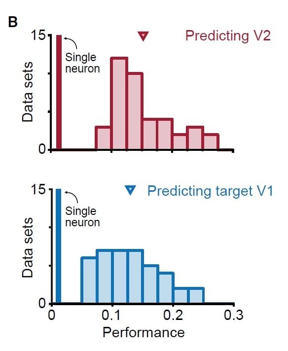 paper, fig 2B (the figure at left) shows the source V1 population activity can predict V2 activity as well as V1 activity can predict its own activity. This was puzzling: we would have thought that it is easier to predict neural activity in the same area because the neurons in the same area may be more interconnected compared to neurons in different areas. We aren’t quite sure about the anatomy here. Perhaps the V1-V1 and V1-V2 connections are similar in amount and strength if all these neurons share overlapped receptive field?

Outlook:

This paper raises an intriguing mechanism for inter-areal interaction: one brain area can project selective information to specific downstream areas through different communication subspaces. Semedo et al. tested this idea on a dataset recorded in anesthetized monkeys. We wonder if this mechanism can be found in awake, and even free-moving animals. Moreover, the authors mainly used a passive grating watching task. But if this is a general mechanism for inter-areal interaction, it would be interesting to look for similar phenomena in more complicated visual tasks and especially multisensory tasks.

Finally, the authors plotted the neuronal activity in a neural space where each axis represents the activity of one neuron. In this case, the weights of all neurons can be represented as a regression dimension across the neural space. If we can keep recording the same neuron group for a long period, we would get the long-term changes of these weights. Then maybe we can use the weights as axes to get a weight space, which shows the change of each neuron’s contribution to the population activity.

References:

1. Semedo, J. D., Zandvakili, A., Machens, C. K., Byron, M. Y., & Kohn, A. (2019). Cortical areas interact through a communication subspace. Neuron, 102(1), 249-259.
2. Kaufman, M. T., Churchland, M. M., Ryu, S. I., & Shenoy, K. V. (2014). Cortical activity in the null space: permitting preparation without movement. Nature neuroscience, 17(3), 440.

 

Shoot, why’d I just do that?

We’ve all had the experience of botching an easy decision. Laboratory subjects, both human and animal, also sometimes make the wrong choice when categorizing stimuli that should be really easy to judge. We recently wrote a paper about this which is on biorxiv. We argued that these lapses are not goof-ups but instead reflect the need for subjects to explore an environment to better understand its rules and rewards. We also made a cake about this finding, which was delicious.

We were happy to hear that Jonathan Pillow‘s lab picked our paper to discuss in their lab meeting. Pillow’s team have, like us, been enthusiastic about new ways to characterize lapses and in fact have a rather interesting (and complimentary account) which you can read if interested. We really enjoyed reading this thoughtful blog by Zoe Ashwood about their lab meeting discussion.

They raised a few concerns which we address below:

Concern #1: The first concern had to do with the probability of attending (), the parameter that determined the overall rate of lapses in the traditional inattention model. We would have liked to see further justification for keeping  the same across the matched and neutral experiments and we question if this is a fair test for the inattention model of lapses. Previous work such as Körding et al. (2007) makes us question whether the animal uses different strategies to solve the task for the matched and neutral experiments. In particular, in the matched experiment, the animal may infer that the auditory and visual stimuli are causally related; whereas in the neutral experiment, the animal may detect the two stimuli as being unrelated. If this is true, then it seems strange to assume that  and  for the inattention model should be the same for the matched and neutral experiments.

 Our response: In the inattention model,  represents the probability of not missing the stimulus – hence it should be influenced by (a) the animal’s attentional state before experiencing the stimulus & (b) the bottom-up salience that allows the stimulus to “pop” into the animal’s attention. Since the matched & neutral stimuli are interleaved and both consisted of equally salient multisensory events, we reasoned that  should be the same on these trials. Also note that even on matched trials, the auditory and visual events are not presented synchronously (the two event streams are independently generated). Surprisingly, this does little to deter a causal inference: animals integrate nonetheless (see Raposo, 2012). So from the point of view of the animal, a trial isn’t obviously a neutral trial right from the outset. In keeping with that, we found that animals were influenced by stimuli over the entire course of the trials, even for neutral trials (see psychophysical kernels below).

But we agree about the different strategies- *after* the animal attends to the stimulus & estimates their rates, it could potentially use this information to infer that a trial is neutral, and should discard the irrelevant visual information (a “causal inference” strategy akin to Kording et. al) rather than integrating it (a “forced fusion” strategy). However, this retrospective discarding differs from inattention because it requires knowledge of the rates and doesn’t produce lapses, instead affecting the – causal inference predicts comparable neutral and auditory sigmas, while forced fusion predicts neutral values of  that are higher than auditory, due to inappropriately integrated noise. Indeed we see comparable neutral and auditory values of  (and values of too), suggesting causal inference.

The second concern had to do with how asymmetric lapses could be accounted for in our new exploration model:

Concern #2 When there are equal rewards for left and right stimuli, is there only a single free parameter determining the lapse rates in the exploration model (namely )? If so, how do the authors allow for asymmetric left and right lapse rates for the exploration model curves of Figure 3e (that is, the upper and lower asymptotes look different for both the matched and neutral curves despite equal left and right reward, yet the exploration model seems able to handle this – how does the model do this?).

Our response: In the exploration model,  in addition to , the lapse rates on either side are determined by the *subjective* values of left and right actions (rL & rR), which must be learnt from experience and hence could be different even when the true rewards are equal, permitting asymmetric lapse rates . When one of the rewards is manipulated, we only allow the corresponding subjective value to change. Since there is an arbitrary scale factor on rR & rL and we only ever manipulate one of the rewards, we can set the un-manipulated reward (say rL) to unity & fit 2 parameters to capture lapses – & rR in units of rL.

The final concern had to do with , the parameter that determined the overall rate of lapses in the exploration model:

Concern #3 How could uncertainty  be calculated by the rat? Can the empirically determined values of  be predicted from, for example, the number of times that the animal has seen the stimulus in the past? And what were some typical values for the parameter  when the exploration model was fit with data? How exploratory were the rats for the different experimental paradigms considered in this paper?

Our response: From the rat’s perspective, can arise naturally as a consequence of Thompson sampling from action value beliefs (Supplementary Fig. 2, also see Gershman 2018) yielding a beta inversely proportional to the root sum of squared variances of action value beliefs. This should also naturally depend on the history of feedback – if the animal receives unambiguous feedback (like sure-bet trials), then these beliefs should be well separated, yielding a higher beta. Supplementary 2 simulates this for 3 levels of sensory noise for a particular sequence of stimuli & a Thompson sampling policy.

On unisensory trials the  values were ~5, meaning that the average uncertainty (S.D.) for unit expected rewards was ~.2, this was reduced to ~.14 on multisensory trials. The near-perfect performance on sure-bet trials suggests negligible uncertainty/exploration on those trials. These values remained unchanged for reward/neural manipulations, which only affected rR/rL depending on the side.

 

ORACLE: June 7, 2019

Today’s paper is, “Simultaneous mesoscopic and two-photon imaging of neuronal activity in cortical circuits”, by Barson D, Hamodi AS, Shen X, Lur G, Constable RT, Cardin JA, Crair MC & Higley MJ. We read this in our lab meeting, and James Roach took the lead on writing it up.

This article brings together two powerful experimental approaches for calcium imaging of cortical activity: 1) using viral injections to the transverse sinus to achieve high GCaMP expression throughout the cortex and thalamus and 2) using a right angle prism and two orthogonal imaging paths to simultaneously capture mesoscale activity from the dorsal cortex and 2-photon single cell activity.

Big Question: How diverse is the cortex-wide functional connectivity of neurons within a local region of the cortex and do these patterns depend on cell type?

Approach: The authors performed mesoscale calcium imaging paired with 2-photon imaging from the primary somatosensory cortex (S1) in awake and behaving mice. Leveraging the novel technical approaches that they introduce here (and [1]), the authors quantify the relationship between the activity of individual cells and populations across the cortex. Using a method similar to spike-triggered-averaging (the cell centered network; CCN), they show that the activity-defined correlations patterns of S1 pyramidal neurons are super diverse (right^*). Interestingly, neurons with similar cortex-wide functional connectivity are not necessarily spatially organized in S1.

To examine whether linkages to cortical networks differ based on cell type and behavioral role, animals expressing td-tomato in VIP⁺ neurons were injected pan-neuronally with GCaMP. VIP⁺ neurons were far more homogeneous in responsiveness to whisking and running behaviors than presumptive pyramidal cells. For both neuron types, membership in cortical networks was predicted by whether the cell was correlated with whisking or running behaviors. These combined effects lead to VIP⁺ neurons being far less diverse than non-VIP⁺ neurons in functional cortical connectivity.

Main take-home: Within a small patch of cortex, the diversity of functional relationship neurons form across the cortex is surprisingly high and that the local spatial arrangement of neurons is not in a “corticotopic map”: two neighboring cells can differ greatly in functional connectivity. The behavioral tuning of a neuron determines, or is the result of, its membership within a functional network. VIP⁺interneurons have a reduced diversity of functional connectivity, but this may be a result of VIP⁺ neurons being more similarly tuned to running or whisking.

Methodologically, this paper makes a significant advance in multiscale recording of neural activity. Pairing 2-photon and mesoscale calcium imaging provides a meaningful advantage in that neuronal cell types can be genetically targeted, cells can be recorded from stably for multiple days, and meso- and microscale activity can be recorded from the same brain region. We were quite impressed by how good the signals from both modalities were (although we would love to see more data comparing the two, especially pixel-by-pixel correlations). Plus, viral injections into the transvers sinus provide for high expression levels without the drawback of other possible sites.

Skeptics Corner:  First, we were a bit concerned that the functional connectivity analysis loses a lot of detail after significance thresholding of the cell centered network data. Preserving some of the complexity in the raw CCN values might support a better alignment to AIBS-defined brain regions. For example cell 2 in figure 3d (below^*) shows peaks in CCN in sensory and motor areas separated by regions with lower correlations, but thresholding for significance leads to these areas being treated equally.

Second, many of the results depend on the functional parcellation of the cortex based upon mesoscale data and we’d love to know a lot more about the outcome of alternative parcellation strategies. Sixteen parcels per hemisphere was chosen to match to number of regions in the Allen CCF,  but how does this parameter affect the analysis? An alternative method, Louvain parcellation (Vanni et al., 2017), does not require the user to specify number of clusters in advance, so we were curious about what that would look like. Also, presenting the functional parcels color-coded for modality implies a bilateral symmetry which is not reliably supported by the borders of the regions (i.e. the hemispheres in figure 3e would look quite different without the color coding). Quantifying the bilateral symmetry of the parcel boundaries would be useful both for  imposing a cost for deviating from symmetry, but also for identifying states or conditions which lead to lateralized cortical activity.

Third, when comparing VIP neurons to putative pyramidal, the distinction of GCaMP+/TdT+ for VIP and GCaMP+/TdT- for pyramidal excludes the possibility that non-VIP interneurons could be expressing GCaMP. Might this contribute to the observed increase in functional diversity for pyramidal neurons reported?

Finally, reporting the cortex-wide functional relationships of the neurons that are not modulated by running or whisking would be an interesting result to add. Are these cells a diverse subset of the S1 population or are they a single functional block?

Outlook: This paper builds on results that highlight the functional diversity of cortical neurons within local circuits. The indication that cell-to-cortex functional relationships can be modulated by behavior highlight that shaping how individual neurons interact with brain wide networks is a central feature of brain states. Multiscale neurophysiology will be a crucial tool in establishing these relationships. An intriguing morsel of information in the article is this: while cell-spiking was uncorrelated with mesoscale activity at a given location, summed spiking and neuropil signal were. This will be important when interpreting a brain region’s mesoscale signal as representing the inputs to, outputs from, or a combination of the two. Mesoscale recordings with soma-targeted calcium reporters (once available) will be useful in disentangling the components of the signal.

*Note we present figure panels from the manuscript with slight modification (cropping) in accordance with the CC BY-NC-ND 4.0 license.

[1] Hamodi A, Martinez Sabino A, Fitzgerald ND, Crair MC (2019) Transverse sinus injections: A novel method for whole-brain vector-driven gene delivery. BioRxiv.

[2] Vanni, M.P., Chan, A.W., Balbi, M., Silasi, G., and Murphy, T.H. (2017). Mesoscale Mapping of Mouse Cortex Reveals Frequency-Dependent Cycling between Distinct Macroscale Functional Modules. J Neurosci37, 7513-7533.